Electrical Noise | Types of Electrical Noise

Electrical noise may be defined as any undesired voltages or currents that ultimately end up appearing in the receiver output. To the listener, this electrical noise often manifests itself as static. It may only be annoying, such as an occasional burst of static, or continuous and of such amplitude that the desired information is obliterated.

Electrical noise signals at their point of origin are generally very small, for example, at the microvolt level. You may be wondering, therefore, why they create so much trouble. Well, a communications receiver is a very sensitive instrument that is given a very small signal at its input that must be greatly amplified before it can drive a speaker.

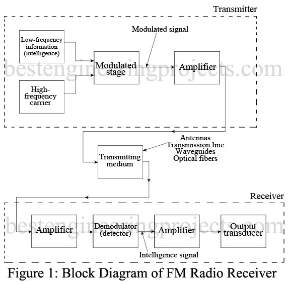
Consider the receiver block diagram shown in Figure 1 to be representative of a standard FM radio (receiver). The first amplifier block, which forms the “front end” of the radio, is required to amplify a received signal from the radio’s antenna that is often less than 10 $\mu V$ . It does not take a very large dose of undesired signal (noise) to ruin reception. This is true even though the transmitter output may be many thousands of watts since when received it is severely attenuated. Therefore, if the desired signal received is of the same order of magnitude as the undesired noise signal, it will probably be unintelligible. This situation is made even worse since the receiver itself introduces additional noise.

Types of Electrical Noise

The noise present in a received radio signal has been introduced in the transmitting medium and is termed external noise. The noise introduced by the receiver is termed internal noise. The important implications of noise considerations in the study of communications systems cannot be overemphasized.

External Electrical Noise

MAN-MADE NOISE: The most troublesome form of external noise is usually the man-made variety. It is often produced by spark-producing mechanisms such as engine ignition systems, fluorescent lights, and commutators in electric motors. This noise is actually “radiated” or transmitted from its generating sources through the atmosphere in the same fashion that a transmitting antenna radiates desirable electrical signals to a receiving antenna. This process is called wave propagation. If the man-made noise exists in the vicinity of the transmitted radio signal and is within its frequency range, these two signals will “add” together. This is an undesirable phenomenon. Man-made noise occurs randomly at frequencies up to around 500 MHz.

Another common source of man-made noise is contained in the power lines that supply the energy for most electronic systems. In this context, the ac ripple in the dc power supply output of a receiver can be classified as noise (an unwanted electrical signal) and must be minimized in receivers that are accepting extremely small intelligence signals. Additionally, ac power lines contain surges of voltage caused by the switching on and off of highly inductive loads such as electrical motors. It is certainly ill-advised to operate sensitive electrical equipment close to an elevator! Man-made noise is weakest in sparsely populated areas, which explains the location of extremely sensitive communications equipment, such as satellite tracking stations, in desert-type locations.

Check out the article on Noise Free Dual Polarity 12V Power Supply Circuit

ATMOSPHERIC NOISE: Atmospheric noise is caused by naturally occurring disturbances in the earth’s atmosphere, with lightning discharges being the most prominent contributors. The frequency content is spread over the entire radio spectrum, but its intensity is inversely related to frequency. It is therefore most troublesome at the lower frequencies. It manifests itself in the static noise that you hear on standard AM radio receivers. Its amplitude is greatest from a storm near the receiver but the additive effect of distant disturbances is also a factor. This is often apparent when listening to a distant station at night on an AM receiver. It is not a significant factor for frequencies exceeding about 20 MHz.

SPACE NOISE: The other form of external noise arrives from outer space and is called space noise. It is pretty evenly divided in origin between the sun and all the other stars. That originating from our star (the sun) is termed solar noise. Solar noise is cyclical and reaches very annoying peaks about every 11 years.

All of the other stars also generate this space noise, and their contribution is termed cosmic noise. Since they are much farther away than the sun, their individual effects are small, but they make up for this by their countless numbers and their additive effects. Space noise occurs at frequencies from about 8 MHz up to 1.5 GHz (1.5 X 10⁹ Hz). While it contains energy at less than 8 MHz, these components are absorbed by the earth’s ionosphere before they can reach the atmosphere. The ionosphere is a region above the atmosphere where free ions and electrons exist in sufficient quantities to have an appreciable effect on wave travel. It includes the area from about 60 to several hundred miles above the earth.

Internal Noise

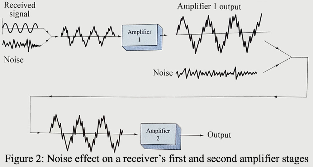
As stated previously, internal noise is introduced by the receiver itself. Thus, the noise already present at the receiving antenna (external noise) has another component added to it before it reaches the output. The receiver’s major noise contribution occurs in its very first stage of amplification. It is there that the desired signal is at its lowest level, and noise injected at that point will be at its largest value in proportion to the intelligence signal. A glance at Figure 2 should help clarify this point. Even though all following stages also introduce noise, their effect is usually negligible concerning the very first stage because of their much higher signal level. Note that the noise injected between amplifiers 1 and 2 has not appreciably increased the noise on the desired signal even though it is of the same magnitude as the noise injected into amplifier 1. For this reason, the first receiver stage must be very carefully designed to have low noise characteristics, with the following stages being decreasingly important as the desired signal gets larger and larger.

THERMAL NOISE: There are two basic types of noise generated by electronic circuits. The first one to consider is due to thermal interaction between the free electrons and vibrating ions in a conductor. It causes the rate of arrival of electrons at either end of a resistor to vary randomly and thereby varies the resistor’s potential difference. Resistors and the resistance within all electronic devices are constantly producing a noise voltage. This form of noise was first thoroughly studied by J. B. Johnson in 1928 and is often termed Johnson noise. Since it is dependent on temperature, it is also referred to as thermal noise. Its frequency content is spread equally throughout the usable spectrum, which leads to a third designator: white noise (from optics, where white light contains all frequencies or colors). The terms Johnson, thermal, and white noise may be used interchangeably. Johnson was able to show that the power of this generated noise is given by

$= P_n = kT \Delta f$ ….(Eq. 1)

Where k = Boltzmann’s constant ( $1.38 \times 10^{-23}J/K$ )

T = resistor temperature in kelvin (K)

$\Delta f$ = frequency bandwidth of the system being considered

Since this noise power is directly proportional to the bandwidth involved, it is advisable to limit a receiver to the smallest bandwidth possible. You may be wondering how the bandwidth figures into this. The noise is an ac voltage that has random instantaneous amplitude but a predictable RMS value. The frequency of this noise voltage is just as random as the voltage peaks. The more frequencies allowed into the measurement (i.e., greater bandwidth) the greater the noise voltage. This means that the RMS noise voltage measured across a resistor is a function of the bandwidth of frequencies included.

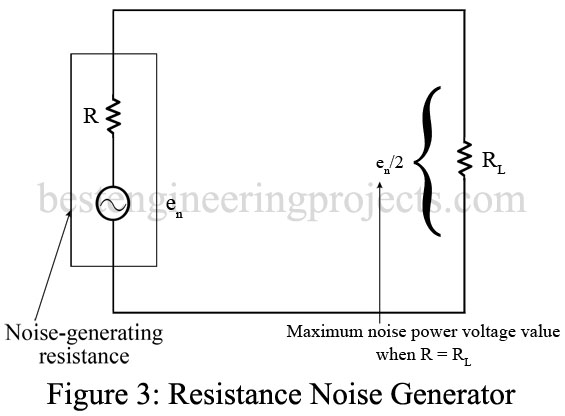
Since $P = \dfrac{E^2}{R}$ , it is possible to rewrite (Eq. 1) to determine the noise voltage ( $e_n$ ) generated by a resistor. Assuming maximum power transfer of the noise source, the noise voltage is split between the load and itself, as shown in Figure 3.

$P_n = \dfrac{(\dfrac{e_n}{2})^2}{R} = kT \Delta f$

Therefore,

$\dfrac{e_n^2}{4} = kT \Delta f R$

$e_n = \sqrt{4 k T \delta f R}$ ……(Eq. 2)

where $e_n$ is the RMS noise voltage and R is the resistance generating the noise. The instantaneous value of thermal noise is not predictable but has peak values generally less than 10 times the RMS value from (Eq. 2). The thermal noise associated with all non-resistor devices is a direct result of their inherent resistance and to a much lesser extent their composition. This applies to capacitors, inductors, and all electronic devices. Equation (2) applies to copper wire-wound resistors, with all other types exhibiting slightly greater noise voltages. Thus, dissimilar resistors of equal value exhibit different noise levels, which gives rise to the term low-noise resistor, which you may have heard before but not understood. Standard carbon resistors are the least expensive variety, but unfortunately, they also tend to be the noisiest. Metal film resistors offer a good compromise in the cost/performance comparison and can be used in all but the most demanding low-noise designs. The ultimate noise performance (lowest noise generated, that is) is obtained with the most expensive and bulkiest variety: the wire-wound resistor. We use (Eq. 2) as a reasonable approximation for all calculations despite these variations.

Example 1: Determine the noise voltage produced by a $1M\Omega$ resistor at room temperature ( $17^0 C$ ) over a 1-MHz bandwidth.

Solution: It is helpful to know that 4kT at room temperature (17°C) is $1.60 \times 10^{-20}$ joules.

$e_n = \sqrt{4kT \Delta f R}$

$= [(1.6 \times 10^{-20})(1 \times 10^6)(1 \times 10^6)]^{\dfrac{1}{2}}$

$= (1.6 \times 10^{-8})^{\dfrac{1}{2}}$

$= 126 \mu V$ rms.

From the preceding example, we can deduce that an ac voltmeter with an input resistance of $1M\Omega$ and a 1-MHz bandwidth generates $126 \mu V$ of noise (RMS). Signals of about $500 \mu V$ or less would certainly not be measured with any accuracy. A $50\Omega$ resistor under the same conditions would generate only about $0.9\mu V$ of noise. This explains why low impedances are desirable in low-noise circuits.

Example 2: An amplifier operating over a 4-MHz bandwidth has a $100\Omega$ input resistance. It is operating at $27^0 C$ , has a voltage gain of 200, and has an input signal of $5\mu V$ . Determine the RMS output signals (desired and noise), assuming external noise can be disregarded.

Solution: To convert °C to kelvin, simply add 273°, so that K = 27°C + 273°C = 300 K. Therefore,

$e_n = \sqrt{4kT \Delta f R}$

$\sqrt{4 \times 1.38 \times 10^{-23} \dfrac{J}{K} \times 300K \times 4MHz \times 100\Omega}$

$= 2.57 \mu V$ rms

After multiplying the input signal $e_s(5 \mu V)$ and noise signal by the voltage gain of 200, the output signal consists of a 1-mV RMS signal and 0.514-mV RMS noise. This is not normally an acceptable situation. The intelligence would probably be unintelligible!

TRANSISTOR NOISE: In Example 2, the noise introduced by the transistor, other than its thermal noise, was not considered. The major contributor to transistor noise is called shot noise. It is due to the discrete-particle nature of the current carriers in all forms of semiconductors. These current carriers, even under de conditions, are not moving in an exactly steady continuous flow since the distance they travel varies due to random paths of motion. The name shot noise is derived from the fact that when amplified into a speaker, it sounds like a shower of lead shot falling on a metallic surface. Shot noise and thermal noise are additive. The equation for shot noise in a diode is

$i_n = \sqrt{2qI_{dc} \Delta f}$ ….(Eq. 3)

Where

$i_n$ = shot noise (rms amperes)

q = electron charge $(1.6 \times 10^{-19}C)$

$I_{dc}$ = dc current (A)

$\delta f$ bandwidth (Hz)

Unfortunately, there is no valid formula to calculate its value for a complete transistor where the sources of shot electrical noise are the currents within the emitter-base and collector-base diodes. Hence, the device user must refer to the manufacturer’s datasheet for an indication of shot noise characteristics. The methods of dealing with these data are covered in Noise Measurement. Shot noise generally increases proportionally with dc bias currents except in MOSFETS, where shot noise seems to be relatively independent of dc current levels.

Example 3:

(a) Determine the shot noise current for a diode with a forward bias of 1 mA over a 100-kHz bandwidth.

(b) Determine the diode’s equivalent noise voltage.

(c) If the diode is in a circuit with 500-ohm series resistance, calculate the total output noise voltage at 27°C.

Solution:

Solution of (a)

$i_n = \sqrt{2qI_{dc} \delta f}$

$= \sqrt{2 \times 1.6 \times 10^{-19} C \times 1 \times 10^{-3} A \times 10^5 Hz}$

$= 0.00566 \mu rms$

Solution of (b)

The dynamic junction resistance of a diode is approximated by the relationship

$R_j \approx \dfrac{26 mV}{I_{dc}}$

$= \dfrac{26 mV}{1 mA} = 26 \Omega$

Therefore, $e_n = i_n \times 26 \Omega$

$= 0.147 \mu V$ rms

Solution of (c)

The noise due to the $5K\Omega$ resistor is

$e_n = \sqrt{4kT \Delta f R}$

$= \sqrt{4 \times 1.38 \times 10^{-23} J/K \times (27 + 273)K \times 10^5 Hz \times 500 \Omega}$

$- 0.91 \mu V$ rms

Therefore,

$i_n = \dfrac{0.91 \mu v rms}{500 \Omega} = 0.00182 \mu A rms$

This current generates a noise voltage across the diode of

$0.00182 \mu A \times 26 \Omega = 0.0473 uV rms$

The total noise voltage of the diode is not the sum of the two sources but is given by the square root of the sum of the squares

$e_{n total} = \sqrt{(0.147 \times 10^{-6})^2 + (0.0473 \times 10^{-6})^2}$

$= 0.154 \mu V$

FREQUENCY NOISE EFFECTS: Two little-understood forms of device noise occur at the opposite extremes of frequency. The low-frequency effect is called excess noise and occurs at frequencies below about 1 kHz. It is inversely proportional to frequency and directly proportional to temperature and dc current levels. It is thought to be caused by crystal surface defects in semiconductors that vary at an inverse rate with frequency. Excess noise is often referred to as flicker noise, pink noise, or 1/f noise. It is present in both bipolar junction transistors (BJT) and field-effect transistors (FET).

At high frequencies, device noise starts to increase rapidly in the vicinity of the device’s high-frequency cutoff. When the transit time of carriers crossing a junction is comparable to the signal’s period (i.e., high frequencies), some of the carriers may diffuse back to the source or emitter. This effect is termed transit-time noise. These high- and low-frequency effects are relatively unimportant in the design of receivers since the critical stages (the front end) will usually be working well above 1 kHz and hopefully below the device’s high-frequency cutoff area. The low-frequency effects are, however, important to the design of low-level, low-frequency amplifiers encountered in certain instrument and biomedical applications.

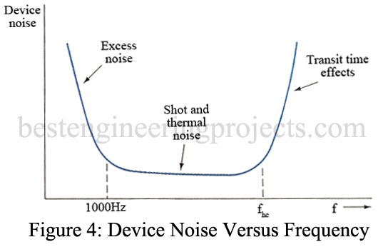
The overall electrical noise intensity versus frequency curves for semiconductor devices (and tubes) have a bathtub shape, as represented in Figure 4. At low frequencies, the excess noise is dominant, while in the midrange shot noise and thermal noise predominate, and above that, the high-frequency effects take over. Of course, tubes are now seldom used and fortunately, their semiconductor replacements offer better noise characteristics. Since semiconductors possess inherent resistances, they generate thermal noise in addition to shot noise, as indicated in Figure 3. The noise characteristics provided in manufacturers’ data sheets take into account both the shot and thermal effects. At the device’s high-frequency cutoff, $f_{hc}$ , the high-frequency effects take over, and the noise increases rapidly.

Types of Electrical Noise

External Electrical Noise

Internal Noise

Share this:

Leave a Comment Cancel reply