Fig.1 (a) shows the free vibration of a system with damping. A device known as damper is shown in the figure below.
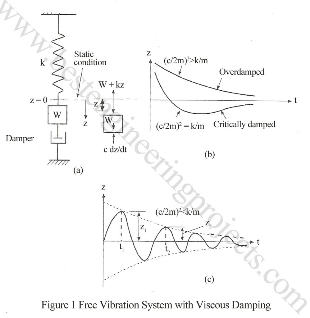
The damping force acts in the opposite direction to that of oscillating mass. The equation of motion for this case can be written as:
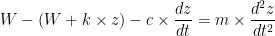 ———-(1)
Where, c = coefficient of viscous damping
Or, 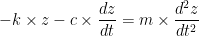 ———-(2)
Or,  ———-(3)
Put  then
then 
And  ———-(4)
By substituting the value in equation (3) we have,
 ———-(5)
The solution for  can be written as:
 ———-(6)
 ———-(7)
The general solution of displacement equation is of the form:
 ———-(8)
The equation (8) will have three possible solutions. They are for (a) real roots, (b) equal roots and (c) imaginary roots.
Real roots 
In this case both roots will be negative and real. Therefore there will be no change in sign and there will be no oscillation and is a case of over damping.
Equal roots 
In this case, both roots will be equal and real. Therefore there will be change in sign once as shown in Fig. 1 (b) and there will be no oscillation and is a case of critical damping. Thus we have,
 ———-(9)
In this case the displacement equation becomes,
 ———-(10)
Imaginary roots 
In this case both roots will be imaginary. The motion will be oscillatory and goes on decaying with time. The general solution of displacement will be derived as follows.
The ratio of  is called damping factor and denoted by D. Thus,
 ———-(11)
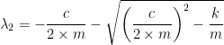
By introducing the relationship for cc, the roots  and
and  becomes,
 ———-(12)
![\lambda_1=\sqrt{\dfrac{k}{m}}\left[-D+i\sqrt{1-D^2}\right]](https://s0.wp.com/latex.php?latex=%5Clambda_1%3D%5Csqrt%7B%5Cdfrac%7Bk%7D%7Bm%7D%7D%5Cleft%5B-D%2Bi%5Csqrt%7B1-D%5E2%7D%5Cright%5D&bg=ffffff&fg=000&s=0&c=20201002)
![\lambda_1=\omega_n\left[-D+i\sqrt{1-D^2}\right]](https://s0.wp.com/latex.php?latex=%5Clambda_1%3D%5Comega_n%5Cleft%5B-D%2Bi%5Csqrt%7B1-D%5E2%7D%5Cright%5D&bg=ffffff&fg=000&s=0&c=20201002) ———-(13)
———-(13)
Similarly, ![\lambda_2=\omega_n\left[-D+i\sqrt{1-D^2}\right]](https://s0.wp.com/latex.php?latex=%5Clambda_2%3D%5Comega_n%5Cleft%5B-D%2Bi%5Csqrt%7B1-D%5E2%7D%5Cright%5D&bg=ffffff&fg=000&s=0&c=20201002) ———-(14)
———-(14)
Putting the values of and in equation (8) we have,
 ———-(15)
![z=C_1\times e^{\omega_n\left[-D+i\sqrt{1-D^2}\right]t}+C_2\times e^{\omega_n\left[-D+i\sqrt{1-D^2}\right]t}](https://s0.wp.com/latex.php?latex=z%3DC_1%5Ctimes+e%5E%7B%5Comega_n%5Cleft%5B-D%2Bi%5Csqrt%7B1-D%5E2%7D%5Cright%5Dt%7D%2BC_2%5Ctimes+e%5E%7B%5Comega_n%5Cleft%5B-D%2Bi%5Csqrt%7B1-D%5E2%7D%5Cright%5Dt%7D&bg=ffffff&fg=000&s=0&c=20201002)
![z=e^{-\omega_nDt}\left[C_1 e^{\omega_ni\sqrt{1-D^2t}} + C_2 e^{-\omega_ni\sqrt{1-D^2t}}\right]](https://s0.wp.com/latex.php?latex=z%3De%5E%7B-%5Comega_nDt%7D%5Cleft%5BC_1+e%5E%7B%5Comega_ni%5Csqrt%7B1-D%5E2t%7D%7D+%2B+C_2+e%5E%7B-%5Comega_ni%5Csqrt%7B1-D%5E2t%7D%7D%5Cright%5D&bg=ffffff&fg=000&s=0&c=20201002)
![z=e^{-\omega_nDt}\left[C_1Cos\left(\omega_n\sqrt{1-D^2t}\right) + iSin\left(\omega_n\sqrt{1-D^2t}\right)+C_2Cos\left(\omega_n\sqrt{1-D^2t}\right) - iSin\left(\omega_n\sqrt{1-D^2t}\right)\right]](https://s0.wp.com/latex.php?latex=z%3De%5E%7B-%5Comega_nDt%7D%5Cleft%5BC_1Cos%5Cleft%28%5Comega_n%5Csqrt%7B1-D%5E2t%7D%5Cright%29+%2B+iSin%5Cleft%28%5Comega_n%5Csqrt%7B1-D%5E2t%7D%5Cright%29%2BC_2Cos%5Cleft%28%5Comega_n%5Csqrt%7B1-D%5E2t%7D%5Cright%29+-+iSin%5Cleft%28%5Comega_n%5Csqrt%7B1-D%5E2t%7D%5Cright%29%5Cright%5D&bg=ffffff&fg=000&s=0&c=20201002)
![z=e^{-\omega_nDt}\left[C_3Sin\left(\omega_n\sqrt{1-D^2t}\right) + C_4Cos\left(\omega_n\sqrt{1-D^2t}\right)\right]](https://s0.wp.com/latex.php?latex=z%3De%5E%7B-%5Comega_nDt%7D%5Cleft%5BC_3Sin%5Cleft%28%5Comega_n%5Csqrt%7B1-D%5E2t%7D%5Cright%29+%2B+C_4Cos%5Cleft%28%5Comega_n%5Csqrt%7B1-D%5E2t%7D%5Cright%29%5Cright%5D&bg=ffffff&fg=000&s=0&c=20201002)
![z=e^{-\omega_nDt}\left[C_3Sin\left(\omega_{Dn}t\right) + C_4Cos\left(\omega_{Dn}t\right)\right]](https://s0.wp.com/latex.php?latex=z%3De%5E%7B-%5Comega_nDt%7D%5Cleft%5BC_3Sin%5Cleft%28%5Comega_%7BDn%7Dt%5Cright%29+%2B+C_4Cos%5Cleft%28%5Comega_%7BDn%7Dt%5Cright%29%5Cright%5D&bg=ffffff&fg=000&s=0&c=20201002) ———-(16)
———-(16)
Where  and it is called damped natural frequency. The natural frequency goes on decreasing with time and the successive peaks can be determined from Fig.1 (c).
Successive peak amplitude
In Fig.1 (c) z1 and z2 are the successive amplitudes and t1 and t2 are the times elapsed. Thus we can write,
 ———-(17)
Hence,
![z_1=e^{-\omega_nDt_1}\left[C_3Sin\left(\omega_{Dn}t_1\right) + C_4Cos\left(\omega_{Dn}t_1\right)\right]](https://s0.wp.com/latex.php?latex=z_1%3De%5E%7B-%5Comega_nDt_1%7D%5Cleft%5BC_3Sin%5Cleft%28%5Comega_%7BDn%7Dt_1%5Cright%29+%2B+C_4Cos%5Cleft%28%5Comega_%7BDn%7Dt_1%5Cright%29%5Cright%5D&bg=ffffff&fg=000&s=0&c=20201002) ———-(18)
———-(18)
![z_2=e^{-\omega_nDt_2}\left[C_3Sin\left(\omega_{Dn}t_2\right) + C_4Cos\left(\omega_{Dn}t_2\right)\right]](https://s0.wp.com/latex.php?latex=z_2%3De%5E%7B-%5Comega_nDt_2%7D%5Cleft%5BC_3Sin%5Cleft%28%5Comega_%7BDn%7Dt_2%5Cright%29+%2B+C_4Cos%5Cleft%28%5Comega_%7BDn%7Dt_2%5Cright%29%5Cright%5D&bg=ffffff&fg=000&s=0&c=20201002) ———-(19)
———-(19)
Again we have,
 ———-(20)

 ———-(21)

 ———-(22)


Therefore, 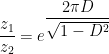 ———-(23)
So the logarithmic decrement is:
 ———-(24)
If D is too small then,  ———-(25)
Thus ratio of successive displacement is constant. If the amplitude decays from z0 to zn over n cycles then,


 ———-(26)