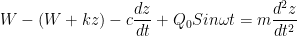
In foundation soil system damping is always present in one form or another. For this case fig. 1 (a), the equation of motion is:


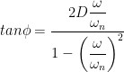
The solution of equation (2) is done by applying the concept of rotating vector. In the figure 1 the exciting force vector Q0 is placed with a phase angle 

In figure 1 (b) the position of motion vector is shown. In figure 1 (c) the position of force vector is shown. The force vectors act opposite to that of motion vectors. The force vector Q0 is placed with a phase angle

And 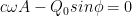
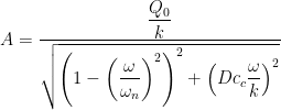
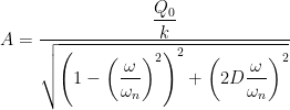
Solving for A and
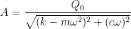
And 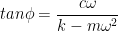


The equations are plotted for various values D as shown in figure 2(a) and (b). These curves are referred to here as response curves for Constant-force-amplitude-excitation. In the figure it is seen that maximum amplitude occurs at a frequency slightly less than the undamped natural circular frequency, 

Resonant frequency at maximum amplitude

Put 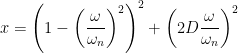


Or,

Or,

Or,

Or,
Or, 
Taking positive sign, we get,

Or, 
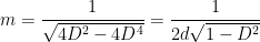
Magnification factor at resonant frequency is given by,

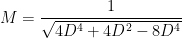
When 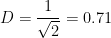
The maximum amplitude at resonance will be,
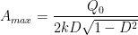
When damping in the system is neglected, then
